Further Analogue-Enhanced Cosimulation including SPICE

⚠️ Warning: This example requires the piel-nix tools environment. See environment configuration documentation.

This example demonstrates the modelling of multi-physical component interconnection and system design.

from piel.models.physical.photonic import (
    mzi2x2_2x2_phase_shifter,
    straight_heater_metal_simple,
)
import hdl21 as h
import pandas as pd
import numpy as np
import piel
import sax
import sys
from gdsfactory.generic_tech import get_generic_pdk
from piel.models.physical.electronic import get_default_models

get_generic_pdk().activate()

Start from gdsfactory

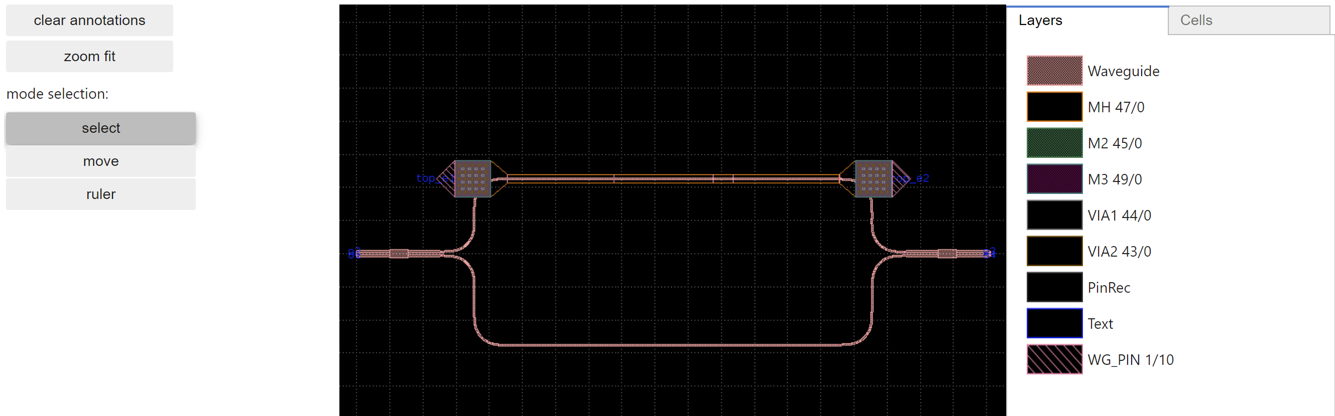
Let us begin from the mzi2x2_2x2_phase_shifter circuit we have been analysing so far in our examples, but this time, we will explore further aspects of the electrical interconnect, and try to extract or extend the simulation functionality. Note that this flattened netlist is the lowest level connectivity analysis, for very computationally complex extraction. Explore the electrical circuit connectivity using the keys below.

mzi2x2_2x2_phase_shifter_netlist_flat = mzi2x2_2x2_phase_shifter().get_netlist_flat( exclude_port_types="optical" ) mzi2x2_2x2_phase_shifter_netlist_flat.keys()

Note that this netlist just gives us electrical connection and connectivity for this component.

mzi2x2_2x2_phase_shifter_netlist_flat["connections"]

The most basic model of this phase-shifter device is treating the heating element as a resistive element. We want to explore how this resistor model affects the rest of the photonic design circuitry. You can already note something important if you explored the netlist with sufficient care and followed the previous examples regarding the straight_x_top or sxt heater component.

mzi2x2_2x2_phase_shifter_netlist = mzi2x2_2x2_phase_shifter().get_netlist(
    exclude_port_types="optical"
)
mzi2x2_2x2_phase_shifter_netlist["instances"]["sxt"]

{'component': 'straight_heater_metal_undercut',
 'info': {'resistance': 0},
 'settings': {'length': 200,
  'length_undercut_spacing': 0,
  'length_undercut': 5,
  'length_straight': 0.1,
  'length_straight_input': 0.1,
  'cross_section': 'xs_sc',
  'cross_section_heater': 'xs_heater_metal',
  'cross_section_waveguide_heater': 'xs_sc_heater_metal',
  'cross_section_heater_undercut': 'xs_sc_heater_metal_undercut',
  'with_undercut': False,
  'via_stack': 'via_stack_heater_mtop',
  'heater_taper_length': 5.0,
  'straight': {'function': 'straight'}}}

So this top heater instance info instance definition, it already includes a resistance field. However, in the default component definition, it is defined as None. Let us give some more details about our circuit, and this would normally be provided by the PDK information of your foundry.

# from gdsfactory.components import straight_heater_metal_simple

our_resistive_mzi_2x2_2x2_phase_shifter = mzi2x2_2x2_phase_shifter()
our_resistive_mzi_2x2_2x2_phase_shifter.plot()

our_resistive_mzi_2x2_2x2_phase_shifter_netlist = (
    our_resistive_mzi_2x2_2x2_phase_shifter.get_netlist(exclude_port_types="optical")
)
our_resistive_mzi_2x2_2x2_phase_shifter_netlist["instances"]["sxt"]

{'component': 'straight_heater_metal_undercut',
 'info': {'resistance': 1000.0},
 'settings': {'cross_section': 'strip',
  'length': 200.0,
  'ohms_per_square': 2,
  'with_undercut': False}}

Now we have a resistance parameter directly connected to the geometry of our phase shifter topology, which is an incredibly powerful tool. In your measurement, you can compute or extract resisivity and performance files parameters of your components in order to create SPICE measurement from them. This is related to the way that you perform your component design. piel can then enable you to understand how this component affects the total system performance.

We can make another variation of our phase shifter to explore physical differences.

our_short_resistive_mzi_2x2_2x2_phase_shifter = mzi2x2_2x2_phase_shifter(
    length_x=100,
)
our_short_resistive_mzi_2x2_2x2_phase_shifter.show()
our_short_resistive_mzi_2x2_2x2_phase_shifter.plot()

You can also find out more information of this component through:

our_short_resistive_mzi_2x2_2x2_phase_shifter.named_references["sxt"].info

Info(resistance=0)

So this is very cool, we have our device model giving us electrical files when connected to the geometrical design parameters. What effect does half that resistance have on the driver though? We need to first create a SPICE model of our circuit. One of the main complexities now is that we need to create a mapping between our component measurement and hdl21 which is dependent on our device model extraction. Another functionality we might desire is to validate physical electrical connectivity by simulating the circuit accordingly.

from gdsfactory.export import to_svg

to_svg(our_short_resistive_mzi_2x2_2x2_phase_shifter)

Extracting the SPICE circuit and assigning model parameters

We will exemplify how piel microservices enable the extraction and configuration of the SPICE circuit. This is done by implementing a SPICE netlist construction backend to the circuit composition functions in sax, and is composed in a way that is then integrated into hdl21 or any SPICE-based solver through the VLSIR Netlist.

The way this is achieved is by extracting all the instances, connections, connection, measurement which is essential to compose our circuit using our piel SPICE backend solver. It follows a very similar principle to all the other sax based circuit composition tools, which are very good.

our_resistive_heater_netlist = straight_heater_metal_simple().get_netlist(
    allow_multiple=True, exclude_port_types="optical"
)
# our_resistive_mzi_2x2_2x2_phase_shifter_netlist = our_resistive_mzi_2x2_2x2_phase_shifter.get_netlist(exclude_port_types="optical")
# our_resistive_heater_netlist

We might want to extract our connections of our gdsfactory netlist, and convert it to names that can directly form part of a SPICE netlist. However, to do this we need to assign what type of element each component each gdsfactory instance is. We show an algorithm that does the following in order to construct our SPICE netlist:

1. Parse the gdsfactory netlist, assign the electrical connection for the model. Extract all instances and required measurement from the netlist.

2. Verify that the measurement have been provided. Each model describes the type of component this is, how many connection it requires and so on. Create a hdl21 top level module for every gdsfactory netlist, this is reasonable as it is composed, and not a generator class. This generates a large amount of instantiated hdl21 modules that are generated from generators.

3. Map the connections to each instance port as part of the instance dictionary. This parses the connectivity in the gdsfactory netlist and connects the connection accordingly.

piel does this for you already:

our_resistive_heater_spice_netlist = (
    piel.integration.gdsfactory_netlist_with_hdl21_generators(
        our_resistive_heater_netlist
    )
)
our_resistive_heater_spice_netlist

This will allow us to create our SPICE connectivity accordingly because it is in a suitable netlist format using hdl21. Each of these components in this netlist is some form of an electrical model or component. We start off from our instance definitions. They are in this format:

our_resistive_heater_netlist["instances"]["straight_1"]

{'component': 'straight',
 'info': {'length': 320.0,
  'width': 0.5,
  'route_info_type': 'xs_sc_heater_metal',
  'route_info_length': 320.0,
  'route_info_weight': 320.0,
  'route_info_xs_sc_heater_metal_length': 320.0},
 'settings': {'length': 320.0,
  'npoints': 2,
  'cross_section': 'xs_sc_heater_metal'},
 'hdl21_model': Generator(name=straight)}

We can compose our SPICE using hdl21 using the measurement we have provided. The final circuit can be extracted accordingly:

our_resistive_heater_circuit = piel.integration.construct_hdl21_module(
    spice_netlist=our_resistive_heater_spice_netlist
)
our_resistive_heater_circuit.instances

{'straight_1': Instance(name=straight_1 of=Module(name=Straight)),
 'taper_1': Instance(name=taper_1 of=Module(name=Taper)),
 'taper_2': Instance(name=taper_2 of=Module(name=Taper)),
 'via_stack_1': Instance(name=via_stack_1 of=Module(name=ViaStack)),
 'via_stack_2': Instance(name=via_stack_2 of=Module(name=ViaStack))}

Note that each component is mapped into hdl21 according to the same structure and names as in the gdsfactory netlist, if you have defined your generator components correctly. Note that the unconnected connection need to be exposed for proper SPICE composition.

our_resistive_heater_circuit.ports

{'e1': Signal(name='e1', width=1, desc=None),
 'e2': Signal(name='e2', width=1, desc=None),
 'via_stack_1__e1': Signal(name='via_stack_1__e1', width=1, desc=None),
 'via_stack_1__e2': Signal(name='via_stack_1__e2', width=1, desc=None),
 'via_stack_1__e4': Signal(name='via_stack_1__e4', width=1, desc=None),
 'via_stack_2__e2': Signal(name='via_stack_2__e2', width=1, desc=None),
 'via_stack_2__e3': Signal(name='via_stack_2__e3', width=1, desc=None),
 'via_stack_2__e4': Signal(name='via_stack_2__e4', width=1, desc=None)}

Same for the signals

our_resistive_heater_circuit.signals

{'via_stack_1_e3': Signal(name='via_stack_1_e3', width=1, desc=None),
 'via_stack_2_e1': Signal(name='via_stack_2_e1', width=1, desc=None)}

We can explore the measurement we have provided too:

We can also extract information for our subinstances. We can also get the netlist of each subinstance using the inherent hdl21 functionality:

h.netlist(
    our_resistive_heater_circuit.instances["straight_1"].of, sys.stdout, fmt="spice"
)

* Anonymous `circuit.Package`
* Generated by `vlsirtools.SpiceNetlister`
*

.SUBCKT Straight
+ e1 e2
* No parameters

rr1
+ e1 e2
+ 1000
* No parameters


.ENDS

One of the main complexities of this translation is that for the SPICE to be generated, the network has to be valid. Sometimes, in direct gdsfactory components, there could be incomplete or undeclared port networks. This means that for the SPICE to be generated, we have to fix the connectivity in some form, and means that there might not be a direct translation from gdsfactory. This is inherently related to the way that the construction of the netlists are generated. This means that to some form, we need to connect the unconnected connection in order for the full netlist to be generated. The complexity is in components such as the via where there are four connection to it on each side. SPICE would treat them as four different inputs that need to be connected.

Now let’s extract the SPICE for our heater circuit:

h.netlist(our_resistive_heater_circuit, sys.stdout, fmt="spice")

* Anonymous `circuit.Package`
* Generated by `vlsirtools.SpiceNetlister`
*

.SUBCKT Straight
+ e1 e2
* No parameters

rr1
+ e1 e2
+ 1000
* No parameters


.ENDS

.SUBCKT Taper
+ e1 e2
* No parameters

rr1
+ e1 e2
+ 1000
* No parameters


.ENDS

.SUBCKT ViaStack
+ e1 e2 e3 e4
* No parameters

rr1
+ e1 e2
+ 1000
* No parameters


rr2
+ e2 e3
+ 1000
* No parameters


rr3
+ e3 e4
+ 1000
* No parameters


rr4
+ e4 e1
+ 1000
* No parameters


.ENDS

.SUBCKT straight_heater_metal_simple_ohms_per_square2
+ e1 e2 via_stack_1__e1 via_stack_1__e2 via_stack_1__e4 via_stack_2__e2 via_stack_2__e3 via_stack_2__e4
* No parameters

xstraight_1
+ e1 e2
+ Straight
* No parameters


xtaper_1
+ via_stack_1_e3 e1
+ Taper
* No parameters


xtaper_2
+ via_stack_2_e1 e2
+ Taper
* No parameters


xvia_stack_1
+ via_stack_1__e1 via_stack_1__e2 via_stack_1_e3 via_stack_1__e4
+ ViaStack
* No parameters


xvia_stack_2
+ via_stack_2_e1 via_stack_2__e2 via_stack_2__e3 via_stack_2__e4
+ ViaStack
* No parameters


.ENDS

So this seems equivalent to the gdsfactory component representation. We can now continue to implement our SPICE simulation.

Flow Automation

piel.flows.extract_component_spice_from_netlist(
    component=straight_heater_metal_simple(),
)

SPICE Integration

We have seen in the previous example how to integrate digital-driven files with photonic circuit steady-state simulations. However, this is making a big assumption: whenever digital codes are applied to photonic components, the photonic component responds immediately. We need to account for the electrical load physics in order to perform more accurate simulation measurement of our systems.

piel provides a set of basic measurement for common photonic loads that integrates closely with gdsfactory. This will enable the multi-domain co-design we like when integrated with all the open-source tools we have previously exemplified. You can find the list and definition of the provided measurement in:

Currently, these measurement do not physically represent electrically the components yet. We will do this later.

piel_hdl21_models = get_default_models()
piel_hdl21_models

We can extract the SPICE out of each model

example_straight_resistor = piel_hdl21_models["straight"]()
h.netlist(example_straight_resistor, sys.stdout, fmt="spice")

* Anonymous `circuit.Package`
* Generated by `vlsirtools.SpiceNetlister`
*

.SUBCKT Straight
+ e1 e2
* No parameters

rr1
+ e1 e2
+ 1000
* No parameters


.ENDS

Creating our Stimulus

Let’s first look into how to map a numpy files into a SPICE waveform. We will create a testbench using the hdl21 interface. So the first thing is that we need to add our stimulus sources, or otherwise where would our pulses come from. We need to construct this into our testbench module. This means we need to generate the connectivity of our signal sources in relation to the connection of our circuit. We create a custom testbench module that we will use to perform this simulation. This needs to contain also our voltage sources for whatever test that we would be performing.

@h.module
class OperatingPointTb:
    """# Basic Extracted Device DC Operating Point Testbench"""

    VSS = h.Port()  # The testbench interface: sole port VSS - GROUND
    VDC = h.Vdc(dc=1)(n=VSS)  # A DC voltage source

    # Our component under test
    dut = example_straight_resistor()
    dut.e1 = VDC.p
    dut.e2 = VSS

In this basic test, we can analyse the DC operating point relationship for this circuit. Now, in order to make these type of simulations more automated to run at scale, piel provides some wrapper functions that can be parameterised with most common simulation parameters:

A Simple DC Operating Point Simulation

simple_operating_point_simulation = (
    piel.tools.hdl21.configure_operating_point_simulation(
        testbench=OperatingPointTb, name="simple_operating_point_simulation"
    )
)
simple_operating_point_simulation

Sim(tb=Module(name=OperatingPointTb), attrs=[Op(name='operating_point_tb')], name='Simulation')

We can now run the simulation using ngpsice. Make sure you have it installed, although this will be automatic in the IIC-OSIC-TOOLS environment:

results = piel.tools.hdl21.run_simulation(simulation=simple_operating_point_simulation)
results

SimResult(an=[OpResult(analysis_name='operating_point_tb', files={'v(xtop.vdc_p)': 1.0, 'i(v.xtop.vvdc)': -0.001})])

We can access the files as a dictionary too:

results.an[0].data

{'v(xtop.vdc_p)': 1.0, 'i(v.xtop.vvdc)': -0.001}

A Simple Transient Simulation

Let’s assume we want to simulate in time how a pulse propagates through our circuit. A resistor on its own will have a linear relationship with the pulse, which means we should see how the current changes from the input pulse in time accordingly. For clarity, we will make a new testbench, even if there are ways to combine them.

@h.module
class TransientTb:
    """# Basic Extracted Device DC Operating Point Testbench"""

    VSS = h.Port()  # The testbench interface: sole port VSS - GROUND
    VPULSE = h.Vpulse(
        delay=1 * h.prefix.m,
        v1=-1000 * h.prefix.m,
        v2=1000 * h.prefix.m,
        period=100 * h.prefix.m,
        rise=10 * h.prefix.m,
        fall=10 * h.prefix.m,
        width=75 * h.prefix.m,
    )(n=VSS)  # A configured voltage pulse source

    # Our component under test
    dut = example_straight_resistor()
    dut.e1 = VPULSE.p
    dut.e2 = VSS

Again we use a simple piel wrapper:

simple_transient_simulation = piel.tools.hdl21.configure_transient_simulation(
    testbench=TransientTb,
    stop_time_s=200e-3,
    step_time_s=1e-4,
    name="simple_transient_simulation",
)
simple_transient_simulation

Sim(tb=Module(name=TransientTb), attrs=[Tran(tstop=0.2*UNIT, tstep=0.0001*UNIT, name='transient_tb')], name='Simulation')

piel.tools.hdl21.run_simulation(simple_transient_simulation, to_csv=True)

When you run the simulation using the piel run_simulation command, there is a to_csv flag that allows us to save the files and access it afterwards. We access the transient simulation in Pandas accordingly:

transient_simulation_results = pd.read_csv("TransientTb.csv")
transient_simulation_results.iloc[20:40]

	Unnamed: 0	time	v(xtop.vpulse_p)	s
20	20	0.00107	-0.986	0.000986
21	21	0.00115	-0.97	0.00097
22	22	0.00125	-0.95	0.00095
23	23	0.00135	-0.93	0.00093
24	24	0.00145	-0.91	0.00091
25	25	0.00155	-0.89	0.00089
26	26	0.00165	-0.87	0.00087
27	27	0.00175	-0.85	0.00085
28	28	0.00185	-0.83	0.00083
29	29	0.00195	-0.81	0.00081
30	30	0.00205	-0.79	0.00079
31	31	0.00215	-0.77	0.00077
32	32	0.00225	-0.75	0.00075
33	33	0.00235	-0.73	0.00073
34	34	0.00245	-0.71	0.00071
35	35	0.00255	-0.69	0.00069
36	36	0.00265	-0.67	0.00067
37	37	0.00275	-0.65	0.00065
38	38	0.00285	-0.63	0.00063
39	39	0.00295	-0.61	0.00061

We can plot our simulation files accordingly:

simple_transient_plot = piel.visual.plot_simple_multi_row(
    data=transient_simulation_results,
    x_axis_column_name="time",
    row_list=[
        "v(xtop.vpulse_p)",
        "i(v.xtop.vvpulse)",
    ],
    y_label=["v(v.xtop.vvpulse)", "i(v.xtop.vvpulse)", "o4 Phase"],
)
simple_transient_plot.savefig(
    "../../_static/img/examples/04_spice_cosimulation/simple_transient_plot.PNG"
)

Extracting Instantaneous Power and Resistance

Now, we have the instantaneous current and voltage at a point in time. You can read some of the documentation in the piel website (TODO LINK) in order to realise the fundamental relationships of this signals. In this circuit, we know that the node v(v.xtop.vvpulse) is at the top of the resistor, and the circuit ground vss is at the bottom. We can read the SPICE netlist to determine this (TODO add automatic schematic mapper). The current i(v.xtop.vvpulse) flows across this resistor according to standard Ohm’s law. So we can extract both the instantaneous power consumption and resistance just from these graphs. Note that this means that these values are subject to insignificant variations from the solver accuracy, so you might want to round to the nearest resistance values for example in some cases.

For this simple example, it is trivial, and we will demonstrate it, but for more complex circuit examples, having a generic framework is important:

transient_simulation_results["power(xtop.vpulse)"] = (
    transient_simulation_results["v(xtop.vpulse_p)"]
    * transient_simulation_results["i(v.xtop.vvpulse)"]
)
transient_simulation_results["resistance(xtop.vpulse)"] = np.round(
    transient_simulation_results["v(xtop.vpulse_p)"]
    / transient_simulation_results["i(v.xtop.vvpulse)"]
)
transient_simulation_results

Note that because the resistance is constant, the power consumption should only vary when there is a change in the signal input. The resistance will always remain constant as the signal voltage and current change, as it is a physical material, and it is easily verified.

transient_simulation_results.iloc[20:40]

	Unnamed: 0	time	v(xtop.vpulse_p)	i(v.xtop.vvpulse)	power(xtop.vpulse)	resistance(xtop.vpulse)
20	20	0.00107	-0.986	0.000986	-0.000972196	1000
21	21	0.00115	-0.97	0.00097	-0.0009409	1000
22	22	0.00125	-0.95	0.00095	-0.0009025	1000
23	23	0.00135	-0.93	0.00093	-0.0008649	1000
24	24	0.00145	-0.91	0.00091	-0.0008281	1000
25	25	0.00155	-0.89	0.00089	-0.0007921	1000
26	26	0.00165	-0.87	0.00087	-0.0007569	1000
27	27	0.00175	-0.85	0.00085	-0.0007225	1000
28	28	0.00185	-0.83	0.00083	-0.0006889	1000
29	29	0.00195	-0.81	0.00081	-0.0006561	1000
30	30	0.00205	-0.79	0.00079	-0.0006241	1000
31	31	0.00215	-0.77	0.00077	-0.0005929	1000
32	32	0.00225	-0.75	0.00075	-0.0005625	1000
33	33	0.00235	-0.73	0.00073	-0.0005329	1000
34	34	0.00245	-0.71	0.00071	-0.0005041	1000
35	35	0.00255	-0.69	0.00069	-0.0004761	1000
36	36	0.00265	-0.67	0.00067	-0.0004489	1000
37	37	0.00275	-0.65	0.00065	-0.0004225	1000
38	38	0.00285	-0.63	0.00063	-0.0003969	1000
39	39	0.00295	-0.61	0.00061	-0.0003721	1000

simple_transient_plot_power_resistance = piel.visual.plot_simple_multi_row(
    data=transient_simulation_results,
    x_axis_column_name="time",
    row_list=[
        "resistance(xtop.vpulse)",
        "power(xtop.vpulse)",
    ],
    y_label=[r"resistance ($\Omega$)", r"power ($W$)"],
)
simple_transient_plot_power_resistance.savefig(
    "../../_static/img/examples/04_spice_cosimulation/simple_transient_plot_power_resistance.PNG"
)

So, we have extracted the power consumption throughout time for pulses we have configured. For the whole period of the simulation, we can extract the energy consumed as the integral of power for a time differential. Note that we expect the energy consumption of this particular circuit, where the resistor is constantly drawing current, to be constantly increasing in time. We can perform a cumulative sum over our power(xtop.vpulse) dataframe which is a discrete integral, and we can multiply that term with the time value to determine the total energy consumption at a point in time.

transient_simulation_results["energy_consumed(xtop.vpulse)"] = (
    transient_simulation_results["power(xtop.vpulse)"]
    * transient_simulation_results["time"].diff()
).cumsum()
transient_simulation_results

simple_energy_consumed_plot = transient_simulation_results.plot(
    x="time", y="energy_consumed(xtop.vpulse)"
)
simple_energy_consumed_plot.get_figure().savefig(
    "../../_static/img/examples/04_spice_cosimulation/simple_energy_consumed_plot.PNG"
)

A full visualisation of the signal is including the cumulative energy use:

simple_transient_plot_full = piel.visual.plot_simple_multi_row(
    data=transient_simulation_results,
    x_axis_column_name="time",
    row_list=[
        "v(xtop.vpulse_p)",
        "i(v.xtop.vvpulse)",
        "resistance(xtop.vpulse)",
        "power(xtop.vpulse)",
        "energy_consumed(xtop.vpulse)",
    ],
    y_label=[r"$V$", r"$A$", r"$\Omega$", r"$W$", r"$J$"],
)
simple_transient_plot_full.savefig(
    "../../_static/img/examples/04_spice_cosimulation/simple_transient_plot_full.PNG"
)

Driving our Phase Shifter

We have demonstrated how we can extract a simple model of a resistor and create different measurement of SPICE simulations. Now, let’s consider how would this affect the photonic performance in a phase-shifter context. One important aspect is that we need to create a mapping between our analogue voltage and a phase. Ideally, this should be a functional mapping.

Let’s create an arbitrary phase mapping with a function that bounds the voltage linearly. What we can do is create a function with a particular phase-power slope. This will vary depending on the thermo-optic modulator design so we will choose an arbitrary value.

def linear_phase_mapping_relationship(
    phase_power_slope: float,
    zero_power_phase: float,
):
    """
    This function returns a function that maps the power applied to a particular heater resistor linearly. For
    example, we might start with a minimum phase mapping of (0,0) where the units are in (Watts, Phase). If we have a ridiculous arbitrary phase_power_slope of 1rad/1W, then the points in our linear mapping would be (0,0), (1,1), (2,2), (3,3), etc. This is implemented as a lambda function that takes in a power and returns a phase. The units of the power and phase are determined by the phase_power_slope and zero_power_phase. The zero_power_phase is the phase at zero power. The phase_power_slope is the slope of the linear mapping. The units of the phase_power_slope are radians/Watt. The units of the zero_power_phase are radians. The units of the power are Watts. The units of the phase are radians.

    Args:
        phase_power_slope (float): The slope of the linear mapping. The units of the phase_power_slope are radians/Watt.
        zero_power_phase (float): The phase at zero power. The units of the zero_power_phase are radians.

    Returns:
        linear_phase_mapping (function): A function that maps the power applied to a particular heater resistor linearly. The units of the power and phase are determined by the phase_power_slope and zero_power_phase. The zero_power_phase is the phase at zero power. The phase_power_slope is the slope of the linear mapping. The units of the phase_power_slope are radians/Watt. The units of the zero_power_phase are radians. The units of the power are Watts. The units of the phase are radians.
    """

    def linear_phase_mapping(power_w: float) -> float:
        """
        We create a linear interpolation based on the phase_power_slope. This function returns phase in radians.
        """
        return phase_power_slope * power_w + zero_power_phase

    return linear_phase_mapping

our_phase_power_map = (
    piel.models.physical.electro_optic.linear_phase_mapping_relationship(
        phase_power_slope=10, zero_power_phase=1
    )
)
power_w_i = np.linspace(0, 1)
linear_phase_power_mapping = piel.visual.plot_simple(
    x_data=power_w_i,
    y_data=our_phase_power_map(power_w=power_w_i),
    ylabel=r"Phase ($\phi$)",
    xlabel=r"Power ($W$)",
)
linear_phase_power_mapping[0].savefig(
    "../../_static/img/examples/04_spice_cosimulation/linear_phase_power_mapping.png"
)

This is all very nice and good, but now we need to map our power in time, to the corresponding phase of our phase shifter. We follow the same principles as the previous digitally-driven modulator example.

our_resistive_mzi_2x2_2x2_phase_shifter_optical_netlist = (
    our_resistive_mzi_2x2_2x2_phase_shifter.get_netlist(exclude_port_types="electrical")
)

mzi2x2_model, mzi2x2_model_info = sax.circuit(
    netlist=our_resistive_mzi_2x2_2x2_phase_shifter_optical_netlist,
    models=piel.models.frequency.get_default_models(),
)

mzi2x2_analogue_active_unitary_array = list()
for power_i in transient_simulation_results["power(xtop.vpulse)"]:
    phase_i = our_phase_power_map(power_w=power_i)
    mzi2x2_active_unitary_i = piel.tools.sax.sax_to_s_parameters_standard_matrix(
        mzi2x2_model(sxt={"active_phase_rad": phase_i}),
        input_ports_order=(
            "o2",
            "o1",
        ),
    )
    mzi2x2_analogue_active_unitary_array.append(mzi2x2_active_unitary_i)
transient_simulation_results["unitary"] = mzi2x2_analogue_active_unitary_array

Note that this operation is very computationally intensive, as we are getting the unitary at every particular point in time within the analog simulation resolution. However, it is reasonable computable within about a minute. We can now see how our optical connection change following the principles in the digital simulation.

optical_port_input = np.array([1, 0])
output_amplitude_array_0 = np.array([])
output_amplitude_array_1 = np.array([])
for unitary_i in transient_simulation_results.unitary:
    output_amplitude_i = np.dot(unitary_i[0], optical_port_input)
    output_amplitude_array_0 = np.append(
        output_amplitude_array_0, output_amplitude_i[0]
    )
    output_amplitude_array_1 = np.append(
        output_amplitude_array_1, output_amplitude_i[1]
    )
transient_simulation_results["output_amplitude_array_0"] = output_amplitude_array_0
transient_simulation_results["output_amplitude_array_1"] = output_amplitude_array_1
transient_simulation_results["output_amplitude_array_0_abs"] = np.abs(
    transient_simulation_results.output_amplitude_array_0
)
transient_simulation_results["output_amplitude_array_0_phase_rad"] = np.angle(
    transient_simulation_results.output_amplitude_array_0
)
transient_simulation_results["output_amplitude_array_0_phase_deg"] = np.angle(
    transient_simulation_results.output_amplitude_array_0, deg=True
)
transient_simulation_results["output_amplitude_array_1_abs"] = np.abs(
    transient_simulation_results.output_amplitude_array_1
)
transient_simulation_results["output_amplitude_array_1_phase_rad"] = np.angle(
    transient_simulation_results.output_amplitude_array_1
)
transient_simulation_results["output_amplitude_array_1_phase_deg"] = np.angle(
    transient_simulation_results.output_amplitude_array_1, deg=True
)
transient_simulation_results

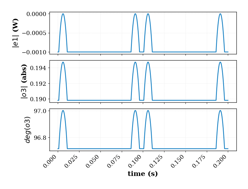
Let’s plot this now:

simple_ideal_o3_mzi_2x2_plots = piel.visual.plot_simple_multi_row(
    data=transient_simulation_results,
    x_axis_column_name="time",
    row_list=[
        "power(xtop.vpulse)",
        "output_amplitude_array_0_abs",
        "output_amplitude_array_0_phase_deg",
    ],
    y_label=[r"$|e1|$ (W)", r"$|o3|$ (abs)", r"$deg(o3)$"],
    x_label="time (s)",
)
simple_ideal_o3_mzi_2x2_plots.savefig(
    "../../_static/img/examples/04_spice_cosimulation/simple_ideal_o3_mzi_2x2_plots.PNG"
)

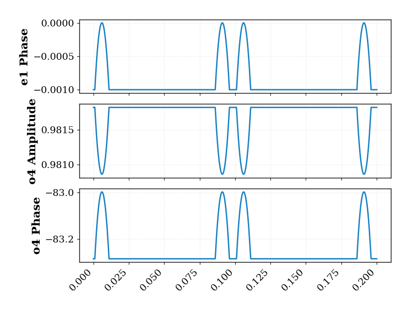
simple_ideal_o4_mzi_2x2_plots = piel.visual.plot_simple_multi_row(
    data=transient_simulation_results,
    x_axis_column_name="time",
    row_list=[
        "power(xtop.vpulse)",
        "output_amplitude_array_1_abs",
        "output_amplitude_array_1_phase_deg",
    ],
    y_label=["e1 Phase", "o4 Amplitude", "o4 Phase"],
)
simple_ideal_o4_mzi_2x2_plots.savefig(
    "../../_static/img/examples/04_spice_cosimulation/simple_ideal_o4_mzi_2x2_plots.PNG"
)

Model Capabilities

We are able to arbitrarily create a model of our devices, and simulate their performance when driven by a particular circuit or not. This is useful as long as our analog model accurately represents the analog performance of our device. It is important, also, to consider opto-physical timing effects not accounted for by transient analog electronic simulations such as thermo-optic relaxation times or carrier-mobility effects. In this case, look into our component-codesign basics example.