Digital Design & Simulation Flow#
⚠️ Warning: This example requires the piel-nix tools environment. See environment configuration documentation.
There are many tools to perform a digital design flow. I have summarised some of the most relevant ones in the TODO LINK INTEGRATION PAGE. In piel, there are a few digital design flow functionalities integrated. However, because the output or interconnections have a set of accepted common measurement, it is possible to use different design flows to integrate with other tools in the flow.
We will explore two popular ones:
amaranthaims to be more than just Python-to-HDL design, but a full digital-flow package design tool.cocotbis mainly used for writing testbenches in Python and verification of logic.
[ ]:
import piel
from piel.types import TruthTable
[ ]:
import simple_design
In this example, we will use amaranth to perform some design and then simulations, so let’s create a suitable project structure based on our initial simple_design, where we will output our files. However, note that the amaranth<0.4 project has of the 23/Ago/2023 a versioning problem which means that they haven’t released a new version for the last two years and this is conflicting with other packages. As such, you have to install the latest amaranth on your own. However, when you
do, you can then run this:
[ ]:
from piel.tools.amaranth import (
    construct_amaranth_module_from_truth_table,
    generate_verilog_from_amaranth_truth_table,
    verify_amaranth_truth_table,
)
[ ]:
# # Uncomment this if you want to run it for the first time.
piel.create_empty_piel_project(
    project_name="amaranth_driven_flow", parent_directory="../designs/"
)
We can also automate the pip installation of our local module:
[ ]:
! pip install -e ../designs/amaranth_driven_flow
#  Uncomment this if you want to run it for the first time.
# piel.pip_install_local_module("../designs/amaranth_driven_flow")
We can check that this has been installed. You might need to restart your jupyter kernel.
[ ]:
import amaranth_driven_flow
[ ]:
amaranth_driven_flow
<module 'amaranth_driven_flow' from 'c:\\users\\dario\\documents\\phd\\piel\\docs\\examples\\designs\\amaranth_driven_flow\\amaranth_driven_flow\\__init__.py'>
amaranth Design Flow#
Let’s design a basic digital module from their example which we can use later. amaranth is one of the great Python digital design flows. I encourage you to check out their documentation for basic examples. We will explore a particular codesign use case: creating bespoke logic for detector optical signals.
Also, another aspect is that amaranth follow a very declarative class-based design flow, which can be tricky to connect with other tools, so piel provides some construction functions that are more easily integrated in the current design flow.
Say we have a table of input optical detector click signals that we want to route some phases to map to some outputs and we want to create a mapping. For now, let’s consider a basic arbitrary truth table in this form:
Input Detector Signals |
Output Phase Map |
|---|---|
00 |
00 |
01 |
10 |
10 |
11 |
11 |
11 |
piel provides some easy functions to perform this convertibility. Say, we provide this information as a dictionary where the keys are the names of our input and output signals. This is a similar principle if you have a detector-triggered DAC bit configuration too.
[ ]:
detector_phase_truth_table_dictionary = {
    "detector_in": ["00", "01", "10", "11"],
    "phase_map_out": ["00", "10", "11", "11"],
}
detector_phase_truth_table = TruthTable(
    input_ports=["detector_in"],
    output_ports=["phase_map_out"],
    **detector_phase_truth_table_dictionary,
)
[ ]:
our_truth_table_module = construct_amaranth_module_from_truth_table(
    truth_table=detector_phase_truth_table
)
amaranth is much easier to use than other design flows like cocotb because it can be purely interacted with in Python, which means there are fewer complexities of integration. However, if you desire to use this with other digital layout tools, for example, OpenROAD as we have previously seen and maintain a coherent project structure with the photonics design flow, piel provides some helper functions to achieve this easily.
We can save this file directly into our working examples directory.
[ ]:
generate_verilog_from_amaranth_truth_table(
    amaranth_module=our_truth_table_module,
    truth_table=detector_phase_truth_table,
    target_file_name="truth_table_module.v",
    target_directory=".",
)
Verilog file generated and written to /home/daquintero/phd/piel/docs/examples/02_digital_design_simulation/our_truth_table_module.v
Another aspect is that as part of the piel flow, we have thoroughly thought of how to structure a codesign electronic-photonic project in order to be able to utilise all the range of tools in the process. You might want to save your design and simulation files to their corresponding locations so you can reuse them with another toolset in the future.
Say, you want to append them to the amaranth_driven_flow project:
[ ]:
design_directory = piel.return_path(amaranth_driven_flow)
Some functions you might want to use to save the designs in these directories are:
[ ]:
amaranth_driven_flow_src_folder = piel.get_module_folder_type_location(
    module=amaranth_driven_flow, folder_type="digital_source"
)
[ ]:
generate_verilog_from_amaranth_truth_table(
    amaranth_module=our_truth_table_module,
    truth_table=detector_phase_truth_table,
    target_file_name="truth_table_module.v",
    target_directory=amaranth_driven_flow_src_folder,
)
Verilog file generated and written to /home/daquintero/phd/piel/docs/examples/designs/amaranth_driven_flow/amaranth_driven_flow/src/truth_table_module.v
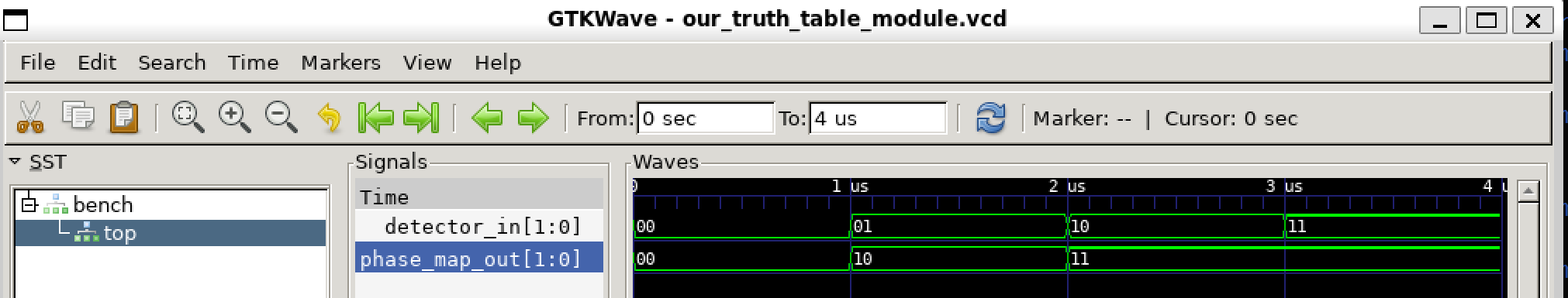
Another thing we can do is verify that our implemented logic is valid. Creating a simulation is also useful in the future when we simulate our extracted place-and-route netlist in relation to the expected applied logic.
[ ]:
verify_amaranth_truth_table(
    truth_table_amaranth_module=our_truth_table_module,
    truth_table=detector_phase_truth_table,
    vcd_file_name="truth_table_module.vcd",
    target_directory=".",
)
VCD file generated and written to /home/daquintero/phd/piel/docs/examples/02_digital_design_simulation/truth_table_module.vcd
You can also use the module directory to automatically save the testbench in these functions.
[ ]:
verify_amaranth_truth_table(
    truth_table_amaranth_module=our_truth_table_module,
    truth_table=detector_phase_truth_table,
    vcd_file_name="truth_table_module.vcd",
    target_directory=amaranth_driven_flow,
)
VCD file generated and written to /home/daquintero/phd/piel/docs/examples/designs/amaranth_driven_flow/amaranth_driven_flow/tb/truth_table_module.vcd
You can observe the design directory of the provided amaranth_driven_flow folder to verify that the files have been included in the other flow.
We can see that the truth table logic has been accurately implemented in the post vcd verification test output generated.
Integration with the openlane v2 flow#
You may want, for example, to layout this design as an openlane design. There are different flows of how to achieve this. We know, for example, that we have a design directory where we want to save the outputs of the openlane runs. It will implement the design using the openlane v2 versions:
[ ]:
from piel.integration.amaranth_openlane import (
    layout_amaranth_truth_table_through_openlane,
)

layout_amaranth_truth_table_through_openlane(
    amaranth_module=our_truth_table_module,
    truth_table=detector_phase_truth_table,
    parent_directory=amaranth_driven_flow,
    openlane_version="v2",
)
[ ]:
from piel.types import TruthTable
import piel

detector_phase_truth_table = {
    "detector_in": ["00", "01", "10", "11"],
    "phase_map_out": ["00", "10", "11", "11"],
}
truth_table = TruthTable(
    input_ports=["detector_in"],
    output_ports=["phase_map_out"],
    **detector_phase_truth_table,
)
am_module = piel.tools.amaranth.construct_amaranth_module_from_truth_table(
    truth_table, logic_implementation_type="sequential"
)
am_module

from piel.integration.amaranth_openlane import (
    layout_amaranth_truth_table_through_openlane,
)

layout_amaranth_truth_table_through_openlane(
    amaranth_module=am_module,
    truth_table=truth_table,
    parent_directory="openlane_run",
    openlane_version="v2",
)
cocotb Simulation#
It is strongly encouraged to get familiar with the piel flow project structure, as this file directory distribution enables the easy use between multiple design tools without conflicts or without structured organisation.
Location of our output files
[ ]:
design_directory = piel.return_path(simple_design)
source_output_files_directory = (
    piel.get_module_folder_type_location(
        module=simple_design, folder_type="digital_source"
    )
    / "out"
)
simulation_output_files_directory = (
    piel.get_module_folder_type_location(
        module=simple_design, folder_type="digital_testbench"
    )
    / "out"
)
simulation_output_files_directory
[ ]:
simulation_output_files_directory.exists()
Check that there exist cocotb python test files already in our design directory:
[ ]:
piel.tools.cocotb.check_cocotb_testbench_exists(simple_design)
Create a cocotb Makefile
[ ]:
piel.tools.cocotb.configure_cocotb_simulation(
    design_directory=simple_design,
    simulator="icarus",
    top_level_language="verilog",
    top_level_verilog_module="adder",
    test_python_module="test_adder",
    design_sources_list=list((design_directory / "src").iterdir()),
)
#!/bin/bash
# Makefile
SIM ?= icarus
TOPLEVEL_LANG ?= verilog
VERILOG_SOURCES += /home/daquintero/phd/piel/docs/examples/designs/simple_design/simple_design/src/adder.vhdl
VERILOG_SOURCES += /home/daquintero/phd/piel/docs/examples/designs/simple_design/simple_design/src/adder.sv
TOPLEVEL := adder
MODULE := test_adder
include $(shell cocotb-config --makefiles)/Makefile.sim
PosixPath('/home/daquintero/phd/piel/docs/examples/designs/simple_design/simple_design/tb/Makefile')
Now we can create the simulation output files from the makefile. Note this will only work in our configured Linux environment.
[ ]:
# Run cocotb simulation
piel.tools.cocotb.run_cocotb_simulation(design_directory)
Standard Output (stdout):
rm -f results.xml
make -f Makefile results.xml
make[1]: Entering directory '/home/daquintero/phd/piel/docs/examples/designs/simple_design/simple_design/tb'
mkdir -p sim_build
/usr/bin/iverilog -o sim_build/sim.vvp -D COCOTB_SIM=1 -s adder  -f sim_build/cmds.f -g2012   /home/daquintero/phd/piel/docs/examples/designs/simple_design/simple_design/src/adder.vhdl  /home/daquintero/phd/piel/docs/examples/designs/simple_design/simple_design/src/adder.sv
rm -f results.xml
MODULE=test_adder  TESTCASE= TOPLEVEL=adder  TOPLEVEL_LANG=verilog  \
         /usr/bin/vvp -M /home/daquintero/.pyenv/versions/3.10.13/envs/piel_0_1_0/lib/python3.10/site-packages/cocotb/libs -m libcocotbvpi_icarus   sim_build/sim.vvp
     -.--ns INFO     gpi                                ..mbed/gpi_embed.cpp:105  in set_program_name_in_venv        Using Python virtual environment interpreter at /home/daquintero/.pyenv/versions/3.10.13/envs/piel_0_1_0/bin/python
     -.--ns INFO     gpi                                ../gpi/GpiCommon.cpp:101  in gpi_print_registered_impl       VPI registered
     0.00ns INFO     cocotb                             Running on Icarus Verilog version 11.0 (stable)
     0.00ns INFO     cocotb                             Running tests with cocotb v1.8.1 from /home/daquintero/.pyenv/versions/3.10.13/envs/piel_0_1_0/lib/python3.10/site-packages/cocotb
     0.00ns INFO     cocotb                             Seeding Python random module with 1718488626
     0.00ns INFO     cocotb.regression                  Found test test_adder.adder_basic_test
     0.00ns INFO     cocotb.regression                  Found test test_adder.adder_randomised_test
     0.00ns INFO     cocotb.regression                  running adder_basic_test (1/2)
                                                          Test for 5 + 10
     2.00ns INFO     cocotb.regression                  adder_basic_test passed
     2.00ns INFO     cocotb.regression                  running adder_randomised_test (2/2)
                                                          Test for adding 2 random numbers multiple times
Example dut.X.value Print
10100
01100
10000
10011
10010
10111
01111
00011
01011
01001
    22.00ns INFO     cocotb.regression                  adder_randomised_test passed
    22.00ns INFO     cocotb.regression                  ******************************************************************************************
                                                        ** TEST                              STATUS  SIM TIME (ns)  REAL TIME (s)  RATIO (ns/s) **
                                                        ******************************************************************************************
                                                        ** test_adder.adder_basic_test        PASS           2.00           0.00       3923.70  **
                                                        ** test_adder.adder_randomised_test   PASS          20.00           0.00       6587.90  **
                                                        ******************************************************************************************
                                                        ** TESTS=2 PASS=2 FAIL=0 SKIP=0                     22.00           0.81         27.25  **
                                                        ******************************************************************************************

VCD info: dumpfile dump.vcd opened for output.
make[1]: Leaving directory '/home/daquintero/phd/piel/docs/examples/designs/simple_design/simple_design/tb'

Standard Error (stderr):
/home/daquintero/phd/piel/docs/examples/designs/simple_design/simple_design/src/adder.vhdl:10: error: Can't find type name `positive'
Encountered 1 errors parsing /home/daquintero/phd/piel/docs/examples/designs/simple_design/simple_design/src/adder.vhdl
However, what we would like to do is extract timing information of the circuit in Python and get corresponding graphs. We would like to have this digital signal information interact with our photonics model. Note that when running a cocotb simulation, this is done through asynchronous coroutines, so it is within the testbench file that any interaction and modelling with the photonics networks is implemented.
Data Visualisation#
The user is free to write their own files visualisation structure and toolset. Conveniently, piel does provide a standard plotting tool for these type of cocotb signal outputs accordingly.
We first list the files for our design directory, which is out simple_design local package if you have followed the correct installation instructions, and we can input our module import rather than an actual path unless you desire to customise.
[ ]:
cocotb_simulation_output_files = (
    piel.tools.cocotb.get_simulation_output_files_from_design(simple_design)
)
cocotb_simulation_output_files
['/home/daquintero/phd/piel/docs/examples/designs/simple_design/simple_design/tb/out/adder_randomised_test.csv']
We can read the simulation output files accordingly:
[ ]:
example_simple_simulation_data = piel.tools.cocotb.read_simulation_data(
    cocotb_simulation_output_files[0]
)
example_simple_simulation_data
Unnamed: 0 |
a |
b |
x |
t |
|
|---|---|---|---|---|---|
0 |
0 |
101 |
1010 |
1111 |
2001 |
1 |
1 |
101 |
1111 |
10100 |
4001 |
2 |
2 |
1000 |
100 |
1100 |
6001 |
3 |
3 |
1000 |
1000 |
10000 |
8001 |
4 |
4 |
1010 |
1001 |
10011 |
10001 |
5 |
5 |
1011 |
111 |
10010 |
12001 |
6 |
6 |
1011 |
1100 |
10111 |
14001 |
7 |
7 |
100 |
1011 |
1111 |
16001 |
8 |
8 |
11 |
0 |
11 |
18001 |
9 |
9 |
110 |
101 |
1011 |
20001 |
10 |
10 |
1 |
1000 |
1001 |
22001 |
Now we can plot the corresponding files using the built-in interactive bokeh signal analyser function:
[ ]:
piel.simple_plot_simulation_data(example_simple_simulation_data)
# TODO fix this properly.
This looks like this:

Sequential Implementation#
[ ]:
try:
    from openlane.flows import SequentialFlow
    from openlane.steps import Yosys, OpenROAD, Magic, Netgen

    class MyFlow(SequentialFlow):
        Steps = [
            Yosys.Synthesis,
            OpenROAD.Floorplan,
            OpenROAD.TapEndcapInsertion,
            OpenROAD.GeneratePDN,
            OpenROAD.IOPlacement,
            OpenROAD.GlobalPlacement,
            OpenROAD.DetailedPlacement,
            OpenROAD.GlobalRouting,
            OpenROAD.DetailedRouting,
            OpenROAD.FillInsertion,
            Magic.StreamOut,
            Magic.DRC,
            Magic.SpiceExtraction,
            Netgen.LVS,
        ]

    flow = MyFlow(
        {
            "PDK": "sky130A",
            "DESIGN_NAME": "spm",
            "VERILOG_FILES": ["./src/spm.v"],
            "CLOCK_PORT": "clk",
            "CLOCK_PERIOD": 10,
        },
        design_dir=".",
    )
    flow.start()
except ModuleNotFoundError as e:
    print(
        f"Make sure you are running this from an environment with Openlane nix installed {e}"
    )